Chapter 4 Categorical data analysis: Preliminaries
Preliminary code
This code is needed to make other code below work:
library(gridExtra) # for grid.arrange() to print plots side-by-side
library(languageR)
library(ggplot2)
library(dplyr)
library(arm)
library(boot)

## loads alternativesMcGillLing620.csv from OSF project for Wagner (2016)
## "Information structure and production planning"
alternatives <- read.delim(url("https://osf.io/6qctp/download"), stringsAsFactors = FALSE)Note: Answers to some questions/exercises not listed in text are in Solutions
4.1 Introduction
So far in this book, we have mostly considered data analysis where the outcome is a continuous variable, like reaction time or vowel duration. In linear regression, the outcome (\(Y\)) is modeled as a function of one or more categorical and continuous predictors (\(X_i\)).
We now turn to categorical data analysis, where the outcome being modeled is a categorical variable. We assume that you have had some exposure to some basic categorical data analysis topics:
Contingency tables (e.g.
xtabsin R)- Including the notion of observed and expected values based on a contingency table, and “observed/expected ratios” (O/E ratios).
Tests of independence of categorical variables
\(\chi^2\) tests
Fisher’s exact test
which we refresh briefly below. If you haven’t seen these topics before, some places to read more are given below.
4.1.1 2x2 contingency tables
Contingency tables show the number of observations for each combination of values of categorical variables. A 2x2 contingency table in particular shows the number of observations for each combination of two categorical variables, \(X_1\) and \(X_2\).
Example
For this subset of the alternatives data:
prominence=AdjectiveorNouncontext=AlternativeorNoAlternative
A contingency table showing the number of observations for each combination of prominence and context:
alternatives.sub <- filter(alternatives, context%in%c('Alternative', 'NoAlternative') &
                               prominence %in% c('Adjective', 'Noun'))
## Warning: package 'bindrcpp' was built under R version 3.4.4xtabs(~prominence + context, data=alternatives.sub)## context
## prominence Alternative NoAlternative
## Adjective 120 55
## Noun 85 155Observed and expected values
In the contingency table above, it looks like prominence isn’t independent of context: Adjective prominence is much more likely relative to Noun prominence in Alternative context. We would like to formally test this hypothesis of non-independence. We can do so using this null hypothesis:
- \(H_0\):
prominenceandcontextoccur independently in this data.
Under \(H_0\), we can work out:
The estimated P(
context=alternative)The estimated P(
prominence=adjective)The expected count in each cell, given the total number of observations \(n\).
For example, for the contingency table above, we can calculate the probabilities #1 and #2:
tab <- xtabs(~prominence + context, data=alternatives.sub)
## total number of observations
n <- sum(tab)

## P(context = alternative)
pAlt <- sum(tab[,'Alternative'])/n

## p(prominence = adjective)
pAdj <- sum(tab['Adjective',])/n

## print these probabilities
pAlt
## [1] 0.4939759pAdj## [1] 0.4216867context=Alternative & prominence=Adjective cell is then:
\[\begin{align}
n \cdot P(`context` = `Alternative`) \cdot P(`prominence` = `Adjective`) & =
415 \cdot 0.4939759 \cdot 0.4216867 \\
& = 86.4457831
\end{align}\]
Exercise 1
Calculate the estimated counts for the other three cells.
4.1.2 The chi-squared test
For a 2x2 contingency table, we have:
The observed counts in each cell, denoted \(O_i\)
The expected counts in each cell, denoted \(E_i\), calculated assuming independence (\(H_0\)).
which measures how much the observed and expected values differ, across the whole contingency table. \(X^2\) is 0 when the observed and expected values are exactly the same, and increases the more the observed and expected values differ.
Pearson’s test statistic approximately follows a \(\chi^2\) distribution (pronounced “chi-squared”) with one degree of freedom, denoted \(\chi^2(1)\), under conditions described below. Thus, we can test the null hypothesis that \(X_1\) and \(X_2\) are independent by comparing the value of \(X^2\) to the \(\chi^2(1)\) distribution.
The same methodology applies for testing independence of two categorical variables with any number of levels. For \(X_1\) and \(X_2\) with \(p\) and \(q\) levels, \(X^2\) can be calculated using Eq. (4.1), and the null hypothesis tested using a \(\chi^2((p-1)(q-1))\) distribution.
Examples
- Are
prominenceandcontextindependent for the contingency table above?
chisq.test(tab)##
## Pearson's Chi-squared test with Yates' continuity correction
##
## data: tab
## X-squared = 43.189, df = 1, p-value = 4.969e-11- Are
RegularityandAuxiliaryindependent in the Dutchregularitydata?
xtabs(~Auxiliary + Regularity, regularity)## Regularity
## Auxiliary irregular regular
## hebben 108 469
## zijn 12 8
## zijnheb 39 64chisq.test(xtabs(~Auxiliary + Regularity, regularity))## Warning in chisq.test(xtabs(~Auxiliary + Regularity, regularity)): Chi-
## squared approximation may be incorrect##
## Pearson's Chi-squared test
##
## data: xtabs(~Auxiliary + Regularity, regularity)
## X-squared = 34.555, df = 2, p-value = 3.136e-08Note that in the regularity example, there is a warning message, related to the “approximately” condition above. The “\(\chi^2\) approximation” (that the test statistic \(X^2\) follows a \(\chi^2\) distribution) is only valid when the expected count in each cell is “big enough”—otherwise, \(p\) values are anti-conservative. Common rules of thumb for “big enough” are 5 or 10 observations per cell.
It is common to have fewer than 10 observations in some cell in a contingency table, making \(\chi^2\) tests frequently inappropriate. Widespread use of the \(\chi^2\) test is to some extent a holdover from when it was computationally difficult to compute “exact” tests (= no approximation to distribution of test statistic), which require simulation, and there is little reason to use the \(\chi^2\) approximation today. For example, you can run a “chi-squared test” but without assuming the \(\chi^2\) approximation by using the simulate.p.value flag to chi.sq:
chisq.test(xtabs(~Auxiliary + Regularity, regularity), simulate.p.value=TRUE)##
## Pearson's Chi-squared test with simulated p-value (based on 2000
## replicates)
##
## data: xtabs(~Auxiliary + Regularity, regularity)
## X-squared = 34.555, df = NA, p-value = 0.0004998which gets rid of the error.
It is still worth knowing about the \(\chi^2\) test and its limitations because it is still frequently used, and in older literature is very widely used. For example, if you are reading a paper where the crucial result relies on a \(\chi^2\) test with \(p=0.02\) for a contingency table with 5 observations in one cell, you should be suspicious. If the contingency table has 20+ observations per cell, you shouldn’t be.
4.1.3 Fisher’s exact test
A good alternative to the \(\chi^2\) test is Fisher’s exact test, which as an “exact test” does not place any assumptions on counts per cell. Fisher’s test asks a slightly different question from a \(\chi^2\) test:
- Given the marginal counts (row and column totals) in the contingency table, if \(X_1\) and \(X_2\) were independent, how likely would an arrangement of the data at least this extreme be?
For example, for testing independence of Auxiliary and Regularity for the Dutch regularity data:
xtabs(~Auxiliary + Regularity, regularity)## Regularity
## Auxiliary irregular regular
## hebben 108 469
## zijn 12 8
## zijnheb 39 64Fisher’s test asks: for 159 irregular verbs, assuming independence, how likely would we be to have \(\geq\) 108 hebben, \(\leq\) 12 zijn, \(\leq\) 39 zijnheb, and so on.
To perform Fisher’s exact test in R:
fisher.test(xtabs(~Auxiliary + Regularity, regularity))##
## Fisher's Exact Test for Count Data
##
## data: xtabs(~Auxiliary + Regularity, regularity)
## p-value = 1.52e-07
## alternative hypothesis: two.sidedAs expected, whether a verb is irregular and which Auxiliary it takes are not independent.
4.2 Towards logistic regression
Intuitively, in logistic regression (next chapter) we will predict the probability that some event happens (e.g. tapping) as a function of predictors, given a bunch of data where each observation corresponds to observing whether the event happened or not, once (\(Y=\) 0 or 1). It would be tempting to just apply the tool we’ve learned so far—linear regression—to this task. However, it’s not obvious what to predict in such a model:
We can’t do a linear regression using \(Y\) as the response, because \(Y\) only takes on the values 0 and 1. We want to model a probability.
However, we can’t do a linear regression using a probability as a response, because (among other reasons) probabilities are bounded by 0 and 1 and linear regression assumes that the response variable can be any number. (We don’t want the model to be able to predict “probability = 2”.)
In order to predict probabilities using a regression model, we need:
Goal 1: A way to think of probabilities on a continuous, unbounded scale.
Goal 2: A way to estimate these probabilities, such that the sample statistic is normally distributed.
Goal 2 is necessary so that we can apply all the statistical inference machinery we have used so far to do things like conduct hypothesis tests.
The answer turns out to be to use “log-odds”, for which we must first discuss “odds”.
4.2.1 Odds
Odds are a way of thinking about probability, as in “how likely is this event to happen versus not happen?”
Questions:
Intuitively, what does it mean to say the odds are 3:1 (“three-to-one”) that it will be sunny tomorrow?
The relationship between probabilities (\(p \in [0,1]\)) and odds are: \[ \text{Odds}(p) = \frac{p}{1 - p} \]
For the example above: if the probability that it is sunny tomorrow is 0.75, then the odds of it being sunny tomorrow are 3 (\(0.75/(1-0.75) = 3\)). The odds of it not being sunny tomorrow are 1/3 (\(0.25/(1-0.25)\)), pronounced “one-to-three”, or “three-to-one against sun tomorrow.”
Figure 4.1 shows odds as a function of probability.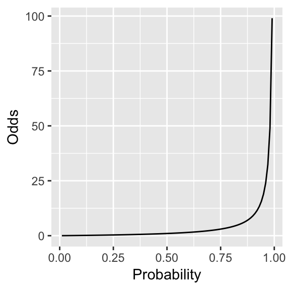
Figure 4.1: Odds as a function of probability.
Odds may be more intuitive than probabilities, but they do not meet Goal 1 (unbounded scale) because odds are always positive.
4.2.2 Log-odds
The log-odds, corresponding to a probability \(p\) are:20 \[ \text{log-odds}(p) = \log \frac{p}{1-p} \] The following figure shows log-odds as a function of probability.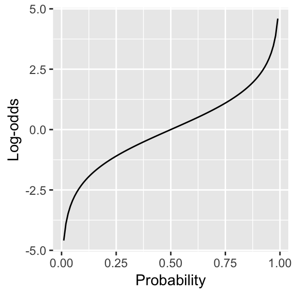
Figure 4.2: Log-odds as a function of probability
Log-odds meet our goals: they range from \(-\infty\) to \(\infty\), and are nearly linear as a function of \(p\), so long as \(p\) isn’t too close to 0 or 1. It also turns out that log-odds satisfy our Goal 2 (normally-distributed sampling statistic), as discussed below.
Log-odds do have an important drawback: they are unintuitive, compared to odds or probability. With some practice you can learn to think in log-odds.
Exercise 2: log-odds practice
What are the log-odds corresponding to these probabilities?
\(p = 0.5\)
\(p = 0.73\)
\(p = 0.88\)
\(p = 0.953\)
## [1] 0## [1] 0.9946226## [1] 1.99243## [1] 3.009467This example illustrates:
Probability space is contracted in log-odds, as we approach 0 or 1: a change of 1 in log-odds corresponds to a smaller and smaller change in \(p\).
Log-odds of -3 to 3 encompasses 90% of probability space (\(\approx p \in (0.05, 0.95)\)).
Note that 4 is huge in log-odds (\(p \approx 0.983\)).
Questions:
What is \(p\) corresponding to log-odds of -4?
## [1] 0.017986214.2.3 Odds ratios
Let’s start with an example from the tapping data, looking at how the likelihood of tapping depends on syntax:
\(Y =\)
tapped(1 = yes, 0 = no)\(X =\)
syntax(1 = transitive, 0 = intransitive)
Suppose that the proportions of cases in each cell for our data are:
\[\begin{array}{c|cc} & Y = 1 & Y = 0 \\ \hline X = 1 & 0.462 & 0.037 \\ X = 0 & 0.43 & 0.07 \end{array}\]We would like a measure of how much more likely tapping is when \(X=1\) than when \(X=0\). One way to do this is to calculate the odds of tapping in each case, then take their ratio:
when \(X = 1\): \(\frac{0.462}{0.037} = 12.49\)
when \(X = 0\): \(\frac{0.43}{0.07} = 6.14\)
Ratio: \(\frac{12.49}{6.14}=\) 2.03
Thus, the odds of tapping are roughly doubled for transitive verbs, relative to intransitive verbs.
To define this odds ratio more generally, suppose that two binary random variables \(X\) and \(Y\) co-occur with these (population) probabilities:
\[\begin{array}{c|cc} & Y = 1 & Y = 0 \\ \hline X = 1 & p_{11} & p_{10} \\ X = 0 & p_{01} & p_{00} \end{array}\]The odds that \(Y=1\) are then:
When \(X = 1\): \(\frac{p_{11}}{p_{10}}\)
When \(X = 0\): \(\frac{p_{01}}{p_{00}}\)
and the odds ratio, as a population statistic, is defined as: \[ OR = \frac{p_{11}/p_{10}}{p_{01}/p_{00}} \]
The odds ratio describes how much the occurrence of one (binary) event depends on another (binary) event, and is often used as an intuitive measure:
“Your odds of developing lung cancer are halved if you quit smoking.”
“Marie’s odds of winning the election tripled from January to March.”
Note that odds ratios are interpreted multiplicatively: it makes sense to say “\(X\) raises the odds of \(Y\) by a factor of 2”, but not “\(X\) raises the odds of \(Y\) by 2”.
Odds ratios are in part a way of thinking about changes in probability. For the tapping example: \[
P(\,\text{tapped}~|~\text{transitive}\,) = 0.926, \quad
P(\,\text{tapped}~|~\text{intransitive}\,) = 0.86
\]
Thus, the change in probability from intransitive to transitive sentences is 0.066. However, odds ratios are not equivalent to changes in probability, because with odds ratios, what a change from \(p\) to \(p + \Delta p\) corresponds to depends on the probability (\(p\)) you start at. For example, Figure 4.3 shows the odds ratio corresponding to a change in probability of 0.1, as a function of the starting probability.
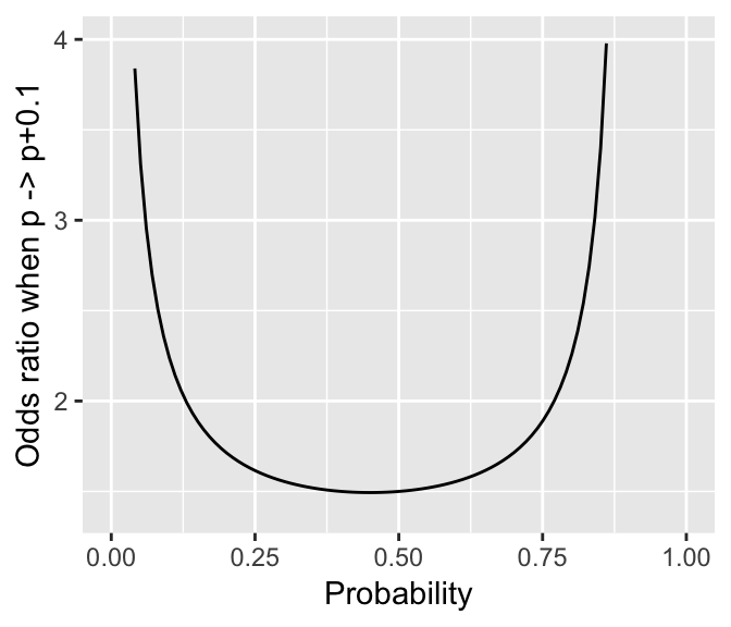
Figure 4.3: Odds ratio when a probability (\(p\)) is increased by 0.1, as a function of \(p\)
For a change in probability from 0.5 to 0.6, the odds increase by about 1.5x, while for a change in probability from 0.85 to 0.95 the odds increase by 3.35x.
To summarize:
Odds have a one-to-one relationship with probabilities
Changes in odds don’t straightforwardly correspond to changes in probabilities.
The non-equivalence between changes in odds and changes in probability is important to remember when interpreting logistic regressions, which are in log-odds space.
4.2.4 Log odds: sample and population
The odds ratio is a useful summary statistic of the degree of dependence between two binary variables, analogous to correlations (\(r\), \(\rho\)) for summarizing dependence between two continuous variables. Because we never actually observe the population value of the odds ratio—which is based on probabilities of each combination of \(X\) and \(Y\)—we need a sample statistic to estimate it from observed counts for each \(X\)/\(Y\) combination.
Suppose we observe the following counts:
\[\begin{array}{c|cc} & Y = 1 & Y = 0 \\ \hline X = 1 & n_{11} & n_{10} \\ X = 0 & n_{01} & n_{00} \end{array}\] To calculate the empirical odds ratio, we estimate each probability from the observed counts. For example: \[\begin{align} P(Y=1|X=1) \approx \frac{n_{11}}{n_{11}+n_{10}}, \quad P(Y=0|X=1) \approx\frac{n_{10}}{n_{11}+n_{10}} \\ \implies Odds(Y=1|X=1) = \frac{n_{11}}{n_{10}} \end{align}\]Similarly estimating \(Odds(Y=1|X=1)\), then taking the logarithm of \(Odds(Y=1|X=1)/Odds(Y=1|X=0)\), gives the sample change in log odds: \[ \hat{L} = \log \left[ \frac{n_{11}/n_{10}}{n_{01}/n_{00}} \right] \]
It turns out that \(\hat{L}\) is normally distributed with mean \(\log(OR)\), where \(OR\) is the population value of the odds ratio. Thus, if we want to do inferential statistics on the effect of binary \(X\) on binary \(Y\), it makes sense to work with log-odds, rather than probabilities.
4.2.4.1 Calculation and interpretation
The function from probability to log-odds is called logit (\(\text{logit}(p)\))
The function from log-odds to probability is called inverse logit (\(\text{logit}^{-1}(x)\)), a.k.a. the “logistic function” (\(1/(1+e^{-x})\)).
Both can be calculated using R functions, such as logit and invlogit in the arm package.
Note that adding in the log-odds scale corresponds to multiplying in the odds scale, by a power of \(e\).
For example, changing log-odds by 1 corresponds to multiplying the odds ratio by \(e\): \[\begin{eqnarray*} \log(OR_1) = 0.69 & \implies & OR_1 = e^{0.69} = 2 \\ \log(OR_2) = 1.69 & \implies & OR_2 = e^{1.69} = 5.42 = 2{\cdot}e \end{eqnarray*}\]Exercise 3
Suppose that in the tapping data, one participant’s tapping rate (i.e. probability of tapping) is 0.90 in fast speech and 0.70 in slow speech.
- What are the participant’s odds of tapping in fast and slow speech (two numbers)?
## [1] 9## [1] 2.333333- What is the odds ratio of tapping (in fast vs. slow speech) (one number)?
## [1] 3.857143- What is the equivalent change in log-odds?
## [1] 1.3499274.3 Other readings
Most introductory statistics books cover contingency tables, chi-squared tests, and Fisher exact tests, including:
General audience: Dalgaard (2008) Ch. 8, Agresti (2007) Ch. 1-2
For psychologists and language scientists: Navarro (2015) Ch. 12, Johnson (2008) Ch. 3.1, 5.1-5.3
The Agresti book is a particularly good and accessible resource for categorical data analysis generally. (Agresti (2003) is Agresti’s more technical/comprehensive book, which is the reference on CDA.)
Some discussion of odds and odds ratios is given by Agresti (2007) Ch. 2, Gelman & Hill (2007) 5.2, Crawley (2015) Ch. 14.
4.4 Solutions
4.4.1 Solutions to Exercise 1:
Estimated Counts for:
Prominence=Noun,Context=Alternativecell = 118.5542Prominence=Adjective,Context=NoAlternativecell = 88.55422Prominence=Adjective,Context=NoAlternativecell = 121.4458
References
Dalgaard, P. (2008). Introductory statistics with R (2nd ed.). New York, NY: Springer.
Agresti, A. (2007). An introduction to categorical data analysis. Wiley.
Johnson, K. (2008). Quantitative methods in linguistics. Malden, MA: Wiley-Blackwell.
Agresti, A. (2003). Categorical data analysis. Wiley.
Gelman, A., & Hill, J. (2007). Data analysis using regression and multilevel/hierarchical models. Cambridge: Cambridge University Press.
Crawley, M. J. (2015). Statistics: an introduction using R (Second edition). Wiley.
Note that \(\log\) here is base \(e\), where \(e=2.718..\) is the base of the natural logarithm.↩