9  Multivariate models

These lecture notes cover topics from:

• Bürkner (2024)

The reading here is short for two reasons, the second more important than the first:

• Students in the 2024 McGill class had a lot to do for the week of these readings
• I’m not aware of any readings on fitting and interpreting multivariate (response) models for linguistic data.

Related readings:

• Barreda and Silbert (2023) Sec. 12.2—discusses multinomial models, which are (under the hood) multivariate models.
• Some sections of McElreath (2020) (and Kurz (2023) translation into brms), e.g. Secs. 5.1.5.3, 11.3.2.1.

Topics:

• Multivariate models: examples
• Intrinsically-related \(y_1\) and \(y_2\)
• Not-IR \(y_1\) and \(y_2\): testing relatedness
  • ``Tying’’ models of \(y_1\) and \(y_2\)
• TODO: Mixture models
  • Data = mixture of \(y_1\) and \(y_2\) distributions
• Coming in a later chapter: mediation
  • \(y_1\) is a predictor of \(y_2\)
  • \(y_1\) mediates the effect of \(x\) on \(y_2\)

9.1 Preliminaries

Load libraries we will need:

library(brms)
library(lme4)
library(arm)
library(tidyverse)

library(tidybayes)

library(bayestestR)

library(phonTools) # TODO

library(patchwork)

# avoids bug where select from MASS is used
select <- dplyr::select

Practical notes

1. If you have loaded rethinking, you need to detach it before using brms. See Kurz (2023) Sec. 4.3.1.

2. I use the file argument when fitting brms models to make compiling this document easier (so the models don’t refit every time I compile). You may or may not want to do this for your own models. See file and file_refit arguments in ?brm.

3. Here I set the file_refit option so “brms will refit the model if model, data or algorithm as passed to Stan differ from what is stored in the file.”

options(brms.file_refit = "on_change")

4. I use chains = 4, cores = 4 when fitting brm models below—this means 4 chains, each to be run on one core on my laptop. cores = 4 may need to be adjusted for your computer. (You may have fewer or more cores; I have 8 cores, so this leaves 50% free.) You should figure out how to use multiple cores on your machine.

5. Make numbers be printed only to 3 digits, for neater output:

options(digits = 3)

9.2 Data

9.2.1 American English vowels

Install the joeysvowels package (Stanley 2020), if you haven’t done so already:

remotes::install_github("joeystanley/joeysvowels")

The joeysvowels package provides a handful of datasets, some subsets of others, that contain formant measurements and other information about the vowels in my own speech. The purpose of the package is to make vowel data easily accessible for demonstrating code snippets when demonstrating working with sociophonetic data.

library(joeysvowels)

midpoints <- mutate(midpoints, dur = end - start)

We’ll use the midpoints dataset: these are measures of F1 and F2 at vowel midpoint for one speaker’s vowels from many words in a controlled context (surrounding coronal consonants): “odd”, “dad”, “sod”, “Todd”, and so on. Standard F1/F2 vowel plot of all data, with 95% ellipses:¹

midpoints %>% ggplot(aes(x = F2, y = F1)) +
  geom_point(aes(color = vowel), size = 0.2) +
  scale_x_reverse() +
  scale_y_reverse() +
  stat_ellipse(level = 0.95, aes(color = vowel))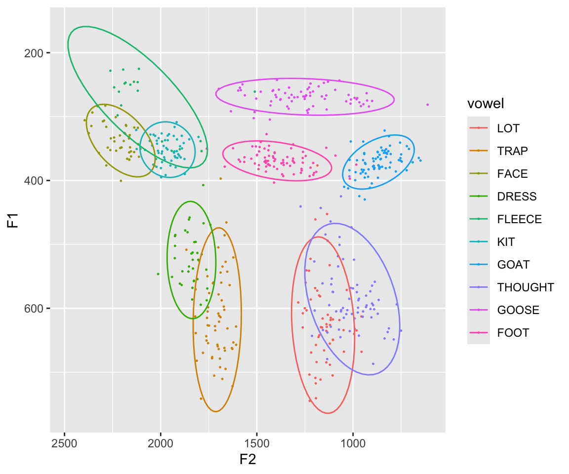

Note how vowel distributions differ both in location (in F1/F2 space) and shape: the direction and size of the ellipse.

Let’s further restrict to just the THOUGHT and LOT vowels for a simple example:

twovowels <- filter(midpoints, vowel %in% c("LOT", "THOUGHT")) %>% droplevels()

RQs for this data could be:

1. Are LOT and THOUGHT pronounced differently?
2. If so, how?

These two vowels are merged for many North American English speakers, but (by self-report) not for this speaker.

Their data for just these vowels looks like:

twovowels %>% ggplot(aes(x = F2, y = F1)) +
  geom_point(aes(color = vowel), size = 0.2) +
  scale_x_reverse() +
  scale_y_reverse() +
  stat_ellipse(level = 0.95, aes(color = vowel))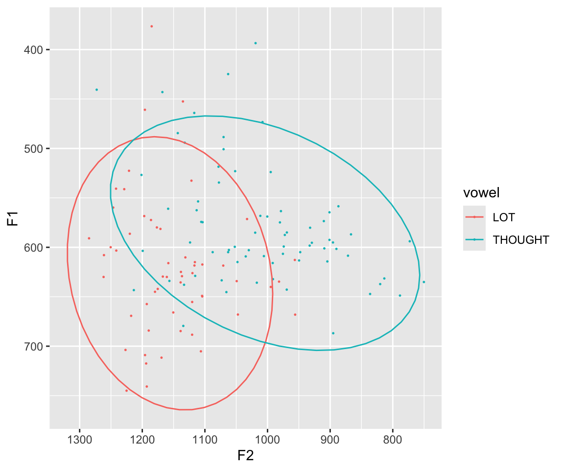

9.2.2 Canadian English voice quality

This is data from a project by Jeanne Brown, a PhD student at McGill (thanks, Jeanne)!

vq_data <- readRDS("jb_creak_data.rds")

This is a greatly simplified subset of the data from from Jeanne’s submitted (paper)[https://papers.ssrn.com/sol3/papers.cfm?abstract_id=4960807] on acoustic measures of “creaky voice” in Canadian English-French bilingual speakers.

This subset is just:

• A couple acoustic measures
• English speech only (the dataset also contains French)
• Only one utterance position (66-99% through utterance)

There are 4884 observations.

Every row corresponds to two acoustic measures that correlate with creaky voice, measured for a single vowel, in a corpus of podcast speech:

• CPP: cepstral peak prominence
  • Continuous, where a lower value is expected to correlate with creakiness.
• bad_f0_track: whether f0 could not be measured for this vowel
  • Binary (0/1), where 1 is expected to correlate with creakiness.

Other columns:

• Sex, Sex_c: factor and (centered) numeric versions of speaker gender (higher = male)
• YOB, YOB_c: raw and normalized (mean/2 SD) year of birth of speaker.
• dev_rate: a measure of speaking rate, relative to the speaker’s mean.
• prev_seg, foll_seg: what kind of segment precede and follow the vowel:
  • vowel, or various consonants (voiceless stop, etc.), or none (= word boundary)

The actual research questions are:

1. Does speaker Sex affect creakiness?
2. Does speaker YOB affect creakiness?

Jeanne’s paper examines these questions on one acoustic measure at a time. We’ll consider a couple additional questions, made possible by jointing modeling the two acoustic measures.

3. Do speakers with higher CPP have a higher probability of bad_f0_track?
4. Do contexts ?

Either one would give insight into whether there is one underlying aspect of voice quality being captured by both measures.

Empirical plots:

p1 <- vq_data %>% group_by(Speaker) %>% mutate(CPP = mean(CPP)) %>% 
  ggplot(aes(x = Sex, y = CPP)) + geom_boxplot() + labs(y = "Speaker average CPP")

p2 <- vq_data %>% group_by(Speaker) %>% mutate(CPP = mean(CPP)) %>% 
  ggplot(aes(x = YOB, y = CPP)) + geom_smooth(method = 'lm') + geom_point() + labs(y = "Speaker average CPP")

p1 + p2
## `geom_smooth()` using formula = 'y ~ x'


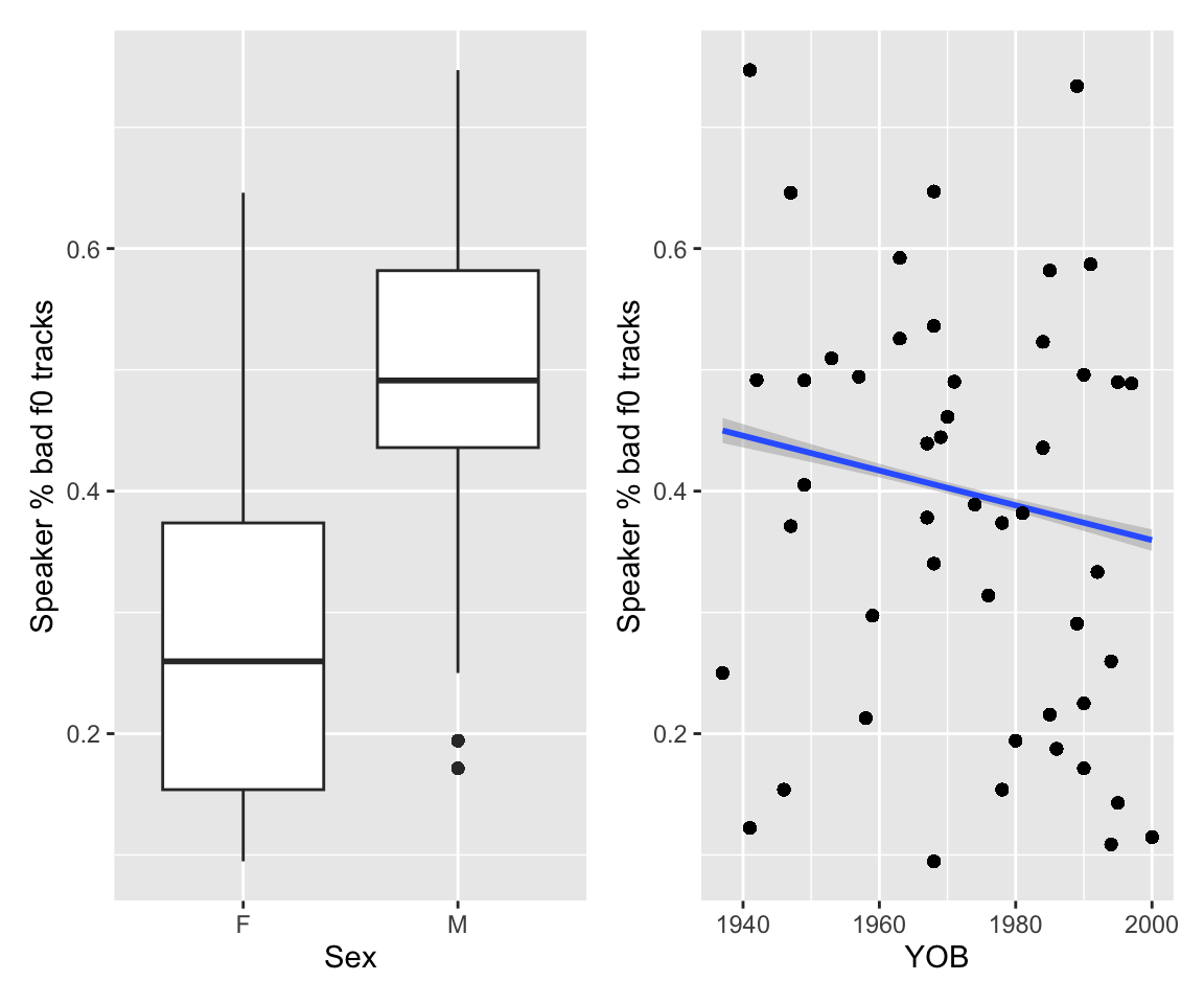
p3 <- vq_data %>% group_by(Speaker) %>% mutate(bt = mean(bad_f0_track)) %>% 
  ggplot(aes(x = Sex, y = bt)) + geom_boxplot() + labs(y = "Speaker % bad f0 tracks")

p4 <- vq_data %>% group_by(Speaker) %>% mutate(bt = mean(bad_f0_track)) %>% 
  ggplot(aes(x = YOB, y = bt)) + geom_smooth(method = 'lm') + geom_point() + labs(y = "Speaker % bad f0 tracks")

p3 + p4
## `geom_smooth()` using formula = 'y ~ x'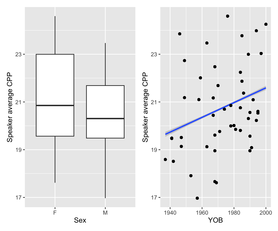

TODO: make similar plots by context

9.3 Intrinsically-related \(y_1\) and \(y_2\)

A multivariate model is one where two or more response variables are modeled simultaneously. In these notes we assume there are just two variables being modeled, called \(y_1\) and \(y_2\).

While the model doesn’t care how \(y_1\) and \(y_2\) are conceptually related, it’s useful to think about different cases:

• \(y_1\) and \(y_2\) are intrinsically related
  • RQs typically about how factors jointly affect \(y_1\) and \(y_2\)
• \(y_1\) and \(y_2\) aren’t intrinsically related
  • RQs can assess whether and how they’re related

An example of the first type is vowel data, which is commonly modeled with at least F1 (first formant) and F2 (second formant). Sometimes F3 and/or duration are included as well.

While F1 and F2 are roughly related to articulatory parameters (jaw opening and tongue backness), this is a rough approximation, and any phonetician would agree that vowels “occur” in multi-dimensional cue space. This is the sense in which F1 and F2 are intrinsically-related.

9.3.1 Independent models

Nonetheless, in analyzing formant data, researchers usually model F1 and F2 are as independent. Let’s do this for the twovowels data, accounting for differences between vowels in location and shape.

To keep our model relatively simple, we’ll assume that shape (parametrized by sigma) doesn’t differ by-word (our data is too sparse to estimate this anyway).

This would be two distributional linear mixed-effects models:

## Include weak priors, so we can calculate Bayes Factors later
##
## Prior: 250 Hz is a large effect for formants
## 15 Hz is a large effect for log
prior_1 <- c(
  prior(normal(0, 250), class = b),
  prior(normal(0, 15), class = b, dpar = sigma)
)

## formula for F1 model
bf1 <- bf(
  F1 ~ vowel,
  sigma ~ vowel
)

## formula for F2 model
bf2 <- bf(
  F2 ~ vowel,
  sigma ~ vowel
)

## Fitting with more iterations than usual, to get OK Bayes factors
## really should be iter = 10k
tv_f1_m1 <- brm(
  formula = bf1, 
  family = gaussian(), 
  data = twovowels, 
  prior = prior_1, 
  chains = 4, cores = 4, iter = 4000, 
  file = "models/tv_f1_m1.brm"
)


tv_f2_m1 <- brm(
  formula = bf2, 
  family = gaussian(), 
  data = twovowels, 
  prior = prior_1, 
  chains = 4, cores = 4, iter = 4000, 
  file = "models/tv_f2_m1.brm"
  )

Model results:

tv_f1_m1
##  Family: gaussian 
##   Links: mu = identity; sigma = log 
## Formula: F1 ~ vowel 
##          sigma ~ vowel
##    Data: twovowels (Number of observations: 127) 
##   Draws: 4 chains, each with iter = 4000; warmup = 2000; thin = 1;
##          total post-warmup draws = 8000
## 
## Regression Coefficients:
##                    Estimate Est.Error l-95% CI u-95% CI Rhat Bulk_ESS Tail_ESS
## Intercept            620.66      9.41   602.32   638.89 1.00     7834     5862
## sigma_Intercept        4.24      0.09     4.07     4.43 1.00     9108     6190
## vowelTHOUGHT         -40.85     11.79   -63.85   -16.97 1.00     8545     5870
## sigma_vowelTHOUGHT    -0.15      0.13    -0.40     0.10 1.00     8927     6271
## 
## Draws were sampled using sampling(NUTS). For each parameter, Bulk_ESS
## and Tail_ESS are effective sample size measures, and Rhat is the potential
## scale reduction factor on split chains (at convergence, Rhat = 1).
tv_f2_m1
##  Family: gaussian 
##   Links: mu = identity; sigma = log 
## Formula: F2 ~ vowel 
##          sigma ~ vowel
##    Data: twovowels (Number of observations: 127) 
##   Draws: 4 chains, each with iter = 4000; warmup = 2000; thin = 1;
##          total post-warmup draws = 8000
## 
## Regression Coefficients:
##                    Estimate Est.Error l-95% CI u-95% CI Rhat Bulk_ESS Tail_ESS
## Intercept           1152.83     10.50  1132.21  1173.36 1.00     9436     6252
## sigma_Intercept        4.34      0.10     4.16     4.55 1.00     8138     5465
## vowelTHOUGHT        -141.12     17.21  -175.02  -107.61 1.00     7131     6459
## sigma_vowelTHOUGHT     0.39      0.13     0.13     0.64 1.00     8158     5818
## 
## Draws were sampled using sampling(NUTS). For each parameter, Bulk_ESS
## and Tail_ESS are effective sample size measures, and Rhat is the potential
## scale reduction factor on split chains (at convergence, Rhat = 1).

Bayes Factors:

bf_pointnull(tv_f1_m1)
## Sampling priors, please wait...
## Warning: Bayes factors might not be precise.
##   For precise Bayes factors, sampling at least 40,000 posterior samples is
##   recommended.
## Bayes Factor (Savage-Dickey density ratio)
## 
## Parameter          |       BF
## -----------------------------
## (Intercept)        | 3.95e+66
## sigma_Intercept    | 7.67e+67
## vowelTHOUGHT       |    15.28
## sigma_vowelTHOUGHT |    0.016
## 
## * Evidence Against The Null: 0
bf_pointnull(tv_f2_m1)
## Sampling priors, please wait...
## Warning: Bayes factors might not be precise.
##   For precise Bayes factors, sampling at least 40,000 posterior samples is
##   recommended.
## Bayes Factor (Savage-Dickey density ratio)
## 
## Parameter          |        BF
## ------------------------------
## (Intercept)        | 4.85e+131
## sigma_Intercept    |  4.86e+55
## vowelTHOUGHT       |  6.53e+08
## sigma_vowelTHOUGHT |     0.696
## 
## * Evidence Against The Null: 0

(These are approximate because we didn’t fit the model for many iterations!)

Answers to our RQs, for F1 and F2 separately:

• Yes, they’re different, in both F1 and F2
• vowel = THOUGHT:
  • lower F1 and F2, much clearer for F2
  • Possible more variable in F2 (95% CredI positive, but BF is inconclusive)

9.3.1.1 Plotting model predictions

Let’s plot model predictions as F1/F2 ellipses, for the LOT and THOUGHT vowels.

For 95% prediction ellipses (like 95% PIs, but in 2D), we first simulate data for each vowel for F1 and F2, separately.²

nd <- data.frame(
  vowel = c("THOUGHT", "LOT")
)
##
f1_samples <- tv_f1_m1 %>%
  add_predicted_draws(newdata = nd, ndraws = 1000) %>%
  dplyr::select(.draw, vowel, F1 = .prediction)
## Adding missing grouping variables: `.row`

f2_samples <- tv_f2_m1 %>%
  add_predicted_draws(newdata = nd, ndraws = 1000) %>%
  dplyr::select(.draw, vowel, F2 = .prediction)
## Adding missing grouping variables: `.row`

These just look like:

f1_samples %>% head()
## # A tibble: 6 × 4
## # Groups:   vowel, .row [1]
##    .row .draw vowel      F1
##   <int> <int> <chr>   <dbl>
## 1     1     1 THOUGHT  621.
## 2     1     2 THOUGHT  560.
## 3     1     3 THOUGHT  551.
## 4     1     4 THOUGHT  597.
## 5     1     5 THOUGHT  643.
## 6     1     6 THOUGHT  568.

Merge F1 and F2 into one dataframe, by matching draws across the two dataframes of predictions:

merged_samples <- inner_join(
  f1_samples,
  f2_samples, 
  by = c(".draw", "vowel")
  ) %>% ## drop irrelevant columns
  select(vowel, F1, F2)

F1/F2 plot with 95% prediction ellipses, over the empirical data:

ggplot(merged_samples, aes(x = F2, y = F1, color = vowel)) +
  geom_point(alpha = 0.5, size = 0.5, data = twovowels) +
  stat_ellipse(level = 0.95) +
  theme_minimal() +
  labs(x = "F1 (Hz)", y = "F2 (Hz)") +
  scale_x_reverse() +
  scale_y_reverse()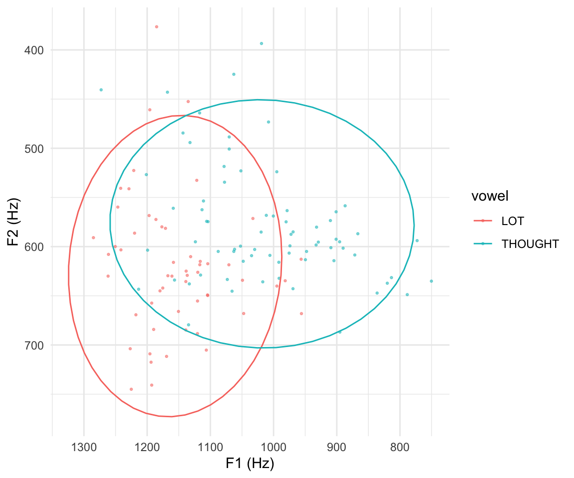

We can do the same procedure to produce 95% credible ellipses by replacing add_predicted_draws() with add_epred_draws() in the code above.

This gives:

f1_samples <- tv_f1_m1 %>%
  add_epred_draws(newdata = nd, ndraws = 1000) %>%
  select(.draw, vowel, F1 = .epred)
## Adding missing grouping variables: `.row`

f2_samples <- tv_f2_m1 %>%
  add_epred_draws(newdata = nd, ndraws = 1000) %>%
  select(.draw, vowel, F2 = .epred)
## Adding missing grouping variables: `.row`

merged_samples <- inner_join(f1_samples, f2_samples, by = c(".draw", "vowel")) %>% ## drop irrelevant columns
  select(vowel, F1, F2)

ggplot(merged_samples, aes(x = F2, y = F1, color = vowel)) +
  stat_ellipse(level = 0.95) +
  theme_minimal() +
  geom_point(alpha = 0.5, size = 0.5, data = twovowels) +
  labs(x = "F1 (Hz)", y = "F2 (Hz)") +
  scale_x_reverse() +
  scale_y_reverse()

The second plot captures visually the result that LOT and THOUGHT are distinct in both F1 and F2: the ellipses are nowhere near overlapping on either axis.

---

This univariate method, where F1 and F2 are analyzed separately, is a perfectly OK way to analyze vowel formant data, but there are a few issues:

• Our RQs are about effects on F1 and F2 jointly (and potentially other acoustic cues, like F3 or duration)—but we are reporting on each one separately.
  • At best, the univariate approach is losing power.
• The models assume that F1 and F2 are uncorrelated—visually, that the F1/F2 ellipses are not tilted in F1/F2 space. We can see that’s not the case from the empirical plot, especially for vowel = THOUGHT.

9.3.2 Multivariate model

We can address these issues by fitting a multivariate model.

## when all response variables have the same
## model structure, can use this shortcut
bf3 <- bf(mvbind(F1, F2) ~ vowel, sigma ~ vowel) +
  set_rescor(TRUE)

## set a very weak prior, so we can calculate Bayes Factors later.
prior_2 <- c(
  prior(normal(0, 250), resp = F1, class = b),
  prior(normal(0, 250), resp = F2, class = b),
  prior(normal(0, 15), class = b, resp = F1, dpar = sigma),
  prior(normal(0, 15), class = b, resp = F2, dpar = sigma)
)

## here we save parameters so we'll be able to calculate
## Bayes Factors versus subset models later.
tv_joint_m1 <- brm(
  formula = bf3,
  family = gaussian(), 
  data = twovowels, 
  chains = 4, cores = 4, iter = 2000, 
  prior = prior_2, 
  save_pars = save_pars(all = TRUE), 
  file = "models/tv_joint_m1.brm"
)

Some notes:

• set_rescor(TRUE): allows the residuals of F1 and F2 to be correlated.
  • This makes sense in the current case (F1 and F2 are intrinsically related), but in other cases (i.e., mediation analyses) won’t necessarily make sense.
    
  • It’s also not possible if one of the models for \(y_1\) or \(y_2\) doesn’t have residuals, as we’ll see later.
• The family argument together with the fact that formula refers to multiple response variables is enough for brms to determine that this is a multivariate linear regression model.

Summary:

tv_joint_m1
##  Family: MV(gaussian, gaussian) 
##   Links: mu = identity; sigma = log
##          mu = identity; sigma = log 
## Formula: F1 ~ vowel 
##          sigma ~ vowel
##          F2 ~ vowel 
##          sigma ~ vowel
##    Data: twovowels (Number of observations: 127) 
##   Draws: 4 chains, each with iter = 2000; warmup = 1000; thin = 1;
##          total post-warmup draws = 4000
## 
## Regression Coefficients:
##                       Estimate Est.Error l-95% CI u-95% CI Rhat Bulk_ESS
## F1_Intercept            620.81      9.48   601.78   639.01 1.00     5663
## sigma_F1_Intercept        4.27      0.10     4.08     4.46 1.00     6424
## F2_Intercept           1152.61     10.40  1132.49  1172.91 1.00     5860
## sigma_F2_Intercept        4.36      0.10     4.19     4.56 1.00     5386
## F1_vowelTHOUGHT         -41.01     11.96   -64.68   -18.06 1.00     5870
## sigma_F1_vowelTHOUGHT    -0.18      0.13    -0.43     0.07 1.00     6934
## F2_vowelTHOUGHT        -140.50     16.94  -174.17  -108.07 1.00     5160
## sigma_F2_vowelTHOUGHT     0.35      0.12     0.10     0.58 1.00     5993
##                       Tail_ESS
## F1_Intercept              3272
## sigma_F1_Intercept        3104
## F2_Intercept              3330
## sigma_F2_Intercept        3249
## F1_vowelTHOUGHT           2995
## sigma_F1_vowelTHOUGHT     2895
## F2_vowelTHOUGHT           2983
## sigma_F2_vowelTHOUGHT     3326
## 
## Residual Correlations: 
##               Estimate Est.Error l-95% CI u-95% CI Rhat Bulk_ESS Tail_ESS
## rescor(F1,F2)    -0.26      0.08    -0.42    -0.10 1.00     6181     3241
## 
## Draws were sampled using sampling(NUTS). For each parameter, Bulk_ESS
## and Tail_ESS are effective sample size measures, and Rhat is the potential
## scale reduction factor on split chains (at convergence, Rhat = 1).

What some regression coefficients mean:

• F1_Intercept: F1 for vowel = LOT
• sigma_F1_Intercept: \(\log(\sigma)\) for vowel = LOT
• sigma_F1_vowelTHOUGHT: difference in \(\log(\sigma)\) between vowel = THOUGHT and LOT.

Another new term is rescor(F1,F2): the correlation between the residuals of F1 and F2. Its interpretation is, “how correlated are F1 and F2, after accounting for other factors [here: word, vowel]”.

Exercise 9.1 For each of the following coefficients: consider the direction of the model’s estimate, as well as whether the 95% CredI overlaps zero. What does this reflect, visually, in the empirical plot of the data in Section 9.2.1?

1. F2_Intercept

2. F1_vowelTHOUGHT

3. rescor(F1,F2)

4. sigma_F2_vowelTHOUGHT

9.3.2.1 Plotting model predictions

To get 95% prediction ellipses, we again simulate data for each vowel:

samples <- tv_joint_m1 %>%
  add_predicted_draws(newdata = nd, ndraws = 1000) %>%
  ## need to turn data from "long" to "wide" format for plotting
  pivot_wider(names_from = .category, values_from = .prediction)

These draws look like:

samples %>% head()
## # A tibble: 6 × 7
## # Groups:   vowel, .row [1]
##   vowel    .row .chain .iteration .draw    F1    F2
##   <chr>   <int>  <int>      <int> <int> <dbl> <dbl>
## 1 THOUGHT     1     NA         NA     1  588. 1077.
## 2 THOUGHT     1     NA         NA     2  567. 1193.
## 3 THOUGHT     1     NA         NA     3  474. 1047.
## 4 THOUGHT     1     NA         NA     4  637.  951.
## 5 THOUGHT     1     NA         NA     5  630.  917.
## 6 THOUGHT     1     NA         NA     6  494.  884.

F1/F2 plot with 95% prediction ellipses, over the empirical data:

ggplot(samples, aes(x = F2, y = F1, color = vowel)) +
  stat_ellipse(level = 0.95) +
  theme_minimal() +
  geom_point(alpha = 0.5, size = 0.5, data = twovowels) +
  labs(x = "F1 (Hz)", y = "F2 (Hz)") +
  scale_x_reverse() +
  scale_y_reverse()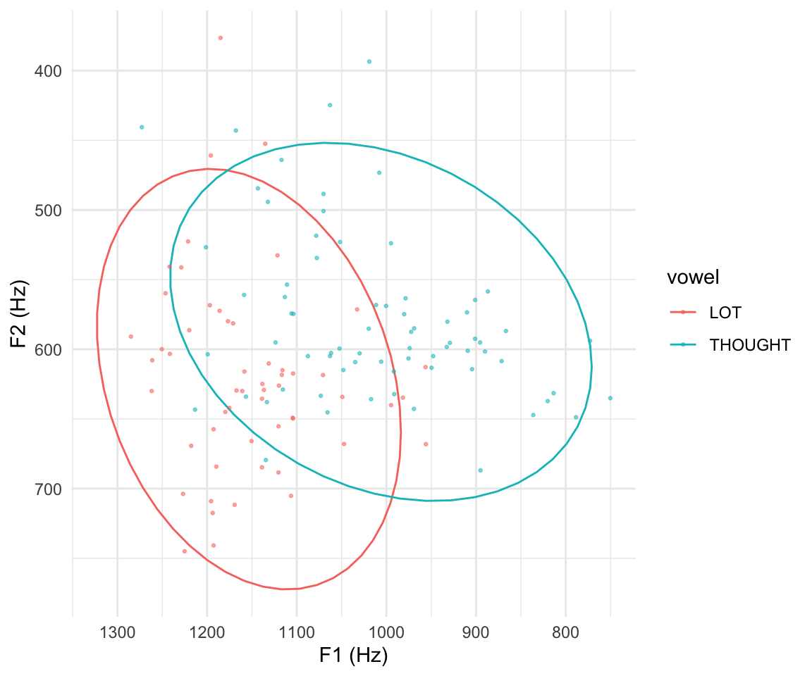

Comparing to the same plot for the univariate model:

• Looks much closer to the empirical plot, compared to model predictions in Section 9.3.1.1.
• Captures the fact that F1 and F2 are not independent, for either LOT or THOUGHT (= ellipses are tilted).

9.3.2.2 Model comparison

The multivariate model also allows us to directly address the question of whether vowel matters, by re-fitting the model without vowel and then comparing the full and subset models.

bf4 <- bf(mvbind(F1, F2) ~ 1, sigma ~ 1) +
  set_rescor(TRUE)

## note: using default prior, prior_2 wouldn't work
tv_joint_m2 <- brm(
  formula = bf4, ,
  family = gaussian(), data = twovowels, chains = 4, cores = 4, iter = 3000, save_pars = save_pars(all = TRUE), file = "models/tv_joint_m2.brm"
)

Model comparison using PSIS-LOO:

tv_joint_m1 <- add_criterion(tv_joint_m1, criterion = "loo", moment_match = TRUE)
tv_joint_m2 <- add_criterion(tv_joint_m2, criterion = "loo", moment_match = TRUE)

loo_compare(tv_joint_m1, tv_joint_m2)
##             elpd_diff se_diff
## tv_joint_m1   0.0       0.0  
## tv_joint_m2 -37.5       8.1

Model comparison using a Bayes Factor:

bayesfactor_models(tv_joint_m2, tv_joint_m1)
## Warning: Bayes factors might not be precise.
##   For precise Bayes factors, sampling at least 40,000 posterior samples is
##   recommended.
## Computation of Marginal Likelihood: estimating marginal likelihood,
##   please wait...
## Computation of Marginal Likelihood: estimating marginal likelihood,
##   please wait...
## Bayes Factors for Model Comparison
## 
##     Model       BF
## [2]       2.91e+11
## 
## * Against Denominator: [1]
## *   Bayes Factor Type: marginal likelihoods (bridgesampling)

LOO and BF addresses RQ1 with a single number: LOT and THOUGHT differ in F1/F2, and the difference is (highly) meaningful.

Exercise 9.2 Make an F1/F2 plot with 95% confidence ellipses for each vowel, for the joint model (tv_joint_m1).

9.4 Assessing relatedness of \(y_1\) and \(y_2\)

We fit a multivariate model of bad_f0_track and CPP for the vq_data dataset, accounting for:

• Both \(y_1\) and \(y_2\) can depend on Sex, YOB_c (RQs 1, 2)

• Speakers can vary in \(y_1\) and \(y_2\)

• The way speakers vary may be correlated between \(y_1\) and \(y_2\) (RQ 3)

• Contexts can vary in \(y_1\) and \(y_2\), i.e., prev_seg and foll_seg

• The way contexts vary may be correlated between \(y_1\) and \(y_2\) (RQ 4)

Model formula:

## just a basic prior for random-effect correlation matrices
prior_1 <- c(
  prior(lkj(1.5), class=cor) 
)


cpp_model <- brmsformula(
  CPP ~  Sex_c + YOB_c+dev_rate  +
    (1 | p | Speaker) +
    (1 | q | prev_seg) +
    (1 | r | foll_seg),
  family = gaussian()
)

bad_f0_track_model <-  brmsformula(bad_f0_track ~  Sex_c + YOB_c+dev_rate  +
  (1 | p | Speaker) +
  (1 | q | prev_seg) +
  (1 | r | foll_seg), family = bernoulli()
) 

joint_model <- cpp_model + bad_f0_track_model + set_rescor(FALSE)

The full model is:

joint_model
## CPP ~ Sex_c + YOB_c + dev_rate + (1 | p | Speaker) + (1 | q | prev_seg) + (1 | r | foll_seg) 
## bad_f0_track ~ Sex_c + YOB_c + dev_rate + (1 | p | Speaker) + (1 | q | prev_seg) + (1 | r | foll_seg)

In this formula, note the | p | |q|, etc. in the random effects. This allows for correlations across random effects for different response variables. For example, (1 | p | Speaker): allows for correlation between by-speaker random intercepts for cpp and bad_track_f0. Its interpretation is, “how correlated are a speaker’s values for these two acoustic cues, after accounting for their Sex and YOB?”

There are four such terms “tying” the two models (for CPP and bad_f0_track) together.

Fit the model:

cpp_badtrack_joint_m1 <- brm(formula = formula_4, 
                             data = PS_sub2 ,
                             chains = 4, cores = 4, iter = 2000,
                             prior = prior_1, 
                             save_pars = save_pars(all = TRUE),
                             file = 'models/cpp_badtrack_joint_m1.brm')

Model summary:

cpp_badtrack_joint_m1
##  Family: MV(gaussian, bernoulli) 
##   Links: mu = identity; sigma = identity
##          mu = logit 
## Formula: CPP ~ Sex_c + YOB_c + dev_rate + (1 | p | Speaker) + (1 | q | prev_seg) + (1 | r | foll_seg) 
##          bad_f0_track ~ Sex_c + YOB_c + dev_rate + (1 | p | Speaker) + (1 | q | prev_seg) + (1 | r | foll_seg) 
##    Data: PS_sub2 (Number of observations: 4884) 
##   Draws: 4 chains, each with iter = 2000; warmup = 1000; thin = 1;
##          total post-warmup draws = 4000
## 
## Multilevel Hyperparameters:
## ~foll_seg (Number of levels: 9) 
##                                         Estimate Est.Error l-95% CI u-95% CI
## sd(CPP_Intercept)                           0.77      0.25     0.43     1.36
## sd(badf0track_Intercept)                    0.63      0.21     0.35     1.15
## cor(CPP_Intercept,badf0track_Intercept)    -0.74      0.22    -0.97    -0.17
##                                         Rhat Bulk_ESS Tail_ESS
## sd(CPP_Intercept)                       1.00     1118     1968
## sd(badf0track_Intercept)                1.00     1338     1923
## cor(CPP_Intercept,badf0track_Intercept) 1.00     1313     1681
## 
## ~prev_seg (Number of levels: 9) 
##                                         Estimate Est.Error l-95% CI u-95% CI
## sd(CPP_Intercept)                           1.07      0.28     0.66     1.76
## sd(badf0track_Intercept)                    1.22      0.32     0.75     2.00
## cor(CPP_Intercept,badf0track_Intercept)    -0.94      0.08    -1.00    -0.69
##                                         Rhat Bulk_ESS Tail_ESS
## sd(CPP_Intercept)                       1.00     1173     1743
## sd(badf0track_Intercept)                1.00     1241     1583
## cor(CPP_Intercept,badf0track_Intercept) 1.00     1347     2259
## 
## ~Speaker (Number of levels: 49) 
##                                         Estimate Est.Error l-95% CI u-95% CI
## sd(CPP_Intercept)                           1.75      0.20     1.40     2.17
## sd(badf0track_Intercept)                    0.71      0.09     0.56     0.91
## cor(CPP_Intercept,badf0track_Intercept)    -0.07      0.15    -0.36     0.23
##                                         Rhat Bulk_ESS Tail_ESS
## sd(CPP_Intercept)                       1.01      622      987
## sd(badf0track_Intercept)                1.00     1206     2052
## cor(CPP_Intercept,badf0track_Intercept) 1.00     1063     1706
## 
## Regression Coefficients:
##                      Estimate Est.Error l-95% CI u-95% CI Rhat Bulk_ESS
## CPP_Intercept           20.51      0.52    19.51    21.54 1.01      692
## badf0track_Intercept    -0.36      0.49    -1.30     0.60 1.00      708
## CPP_Sex_c               -0.99      0.51    -1.97     0.02 1.00      668
## CPP_YOB_c                1.15      0.53     0.08     2.20 1.01      631
## CPP_dev_rate            -0.15      0.04    -0.23    -0.08 1.00     4965
## badf0track_Sex_c         1.14      0.22     0.70     1.57 1.01     1040
## badf0track_YOB_c        -0.32      0.22    -0.77     0.09 1.00     1232
## badf0track_dev_rate     -0.08      0.03    -0.15    -0.03 1.00     5514
##                      Tail_ESS
## CPP_Intercept            1085
## badf0track_Intercept     1237
## CPP_Sex_c                1283
## CPP_YOB_c                1137
## CPP_dev_rate             2877
## badf0track_Sex_c         1511
## badf0track_YOB_c         1686
## badf0track_dev_rate      3238
## 
## Further Distributional Parameters:
##           Estimate Est.Error l-95% CI u-95% CI Rhat Bulk_ESS Tail_ESS
## sigma_CPP     2.80      0.03     2.74     2.86 1.00     5244     2597
## 
## Draws were sampled using sampling(NUTS). For each parameter, Bulk_ESS
## and Tail_ESS are effective sample size measures, and Rhat is the potential
## scale reduction factor on split chains (at convergence, Rhat = 1).

A new type of term here are the random-effect correlations corresponding to different models.

cor(CPP_Intercept,badf0track_Intercept) is the correlation between by-speaker random intercepts for cpp and bad_track_f0.

Exercise 9.3  

1. Which terms in the model address RQs 1 and 2? What answers does it suggest?

2. Which terms in the model address RQs 3 and 4? What answers do they suggest?

3. Consider the effect of foll_seg. Which following contexts give the most and least creakiness (= higher bad_f0_track, lower CPP)? Can you think of why these make (phonetic) sense?

Barreda, Santiago, and Noah Silbert. 2023. Bayesian Multilevel Models for Repeated Measures Data: A Conceptual and Practical Introduction in r. Taylor & Francis. https://santiagobarreda.com/bmmrmd/.

Bürkner, Paul-Christian. 2024. “Estimating Multivariate Models with Brms.” https://cran.r-project.org/web/packages/brms/vignettes/brms_multivariate.html.

Kurz, S. 2023. Statistical Rethinking (Second Edition) with Brms, Ggplot2, and the Tidyverse. https://bookdown.org/content/4857/.

McElreath, Richard. 2020. Statistical Rethinking: A Bayesian Course with Examples in R and Stan. Second. Chapman; Hall/CRC.

Stanley, Joey. 2020. Joeysvowels: Datasets Based on My Speech. https://github.com/joeystanley/joeysvowels.

---

1. If you’re not familiar with these kinds of plot: \(x\) and \(y\) axes go from larger to smaller.

2. Note that these data actually come from different words (column word), so our model should include random effects. I haven’t included random effects just to get the models to fit faster, for pedagogical purposes, and because there are very few observations here anyway (127) relative to model complexity